3.1. Contour-Plot of backscattering matrix

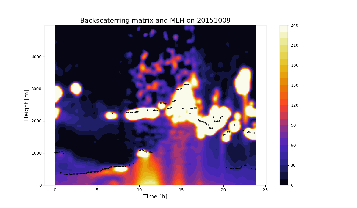
The gallery is capable of transforming Python files into reStructuredText files with a notebook structure. This will allow us to show how to plot the backscattering matrix and add the MLH as dots.

This will make use of the functions to read the matrix (readmatrixfile()), read the MLH file (readmlh()). Both functions are part of the wavelets() module.

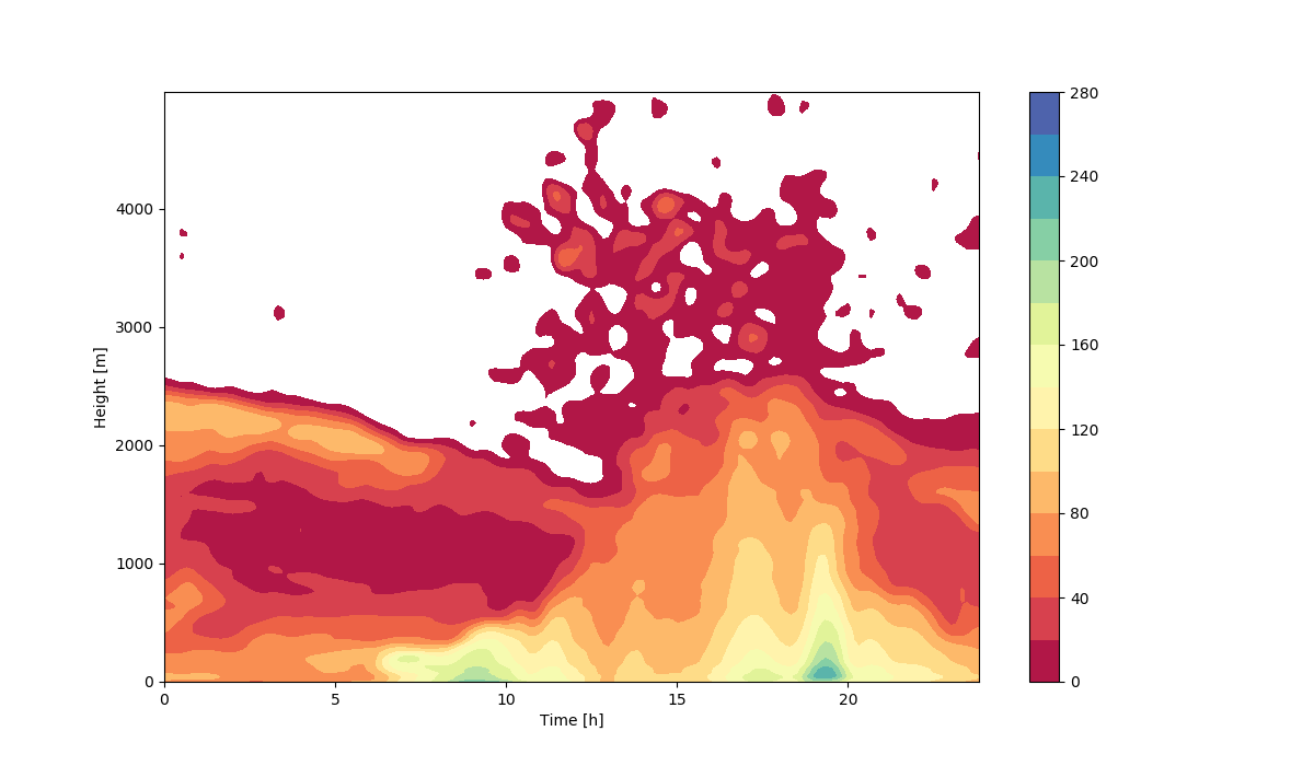
As part of this example, the backscattering matrix is plotted through a contour-plot and MLH through scatter plot. Firstly, we import numpy, matplotlib and the files.

# Code source: JLGF

import numpy as np
import matplotlib.pyplot as plt
from ceilotools import readmatrixfile, readmlh
matrixfile='/home/jlgf/Documents/Python/scripts/20160212_UNAM_prf.txt'
mlhfile='/home/jlgf/Documents/Python/scripts/20160212_UNAM_mlh.txt'

After having established the paths, we read-in both the backscattering matrix and the MLH vectors. Before plotting, a standard procedure is to normalize all values to a maximum and minimum pre-determined level of backscattering. Usually done because at certain heights, backscattering can become zero.

z,time,allprf=readmatrixfile(matrixfile)
mlhtime,mlh=readmlh(mlhfile)
levels=np.arange(0,300,20)
for i in range(len(allprf[0,:])):
  for j in range(len(allprf[:,0])):
    if allprf[j,i] > max(levels):
      allprf[j,i] = max(levels)
    elif allprf[j,i] < min(levels):
      allprf[j,i] = min(levels)
plt.figure(figsize=(12,7))
plt.contourf(time,z,allprf,cmap='Spectral',levels=levels)
plt.colorbar()
plt.scatter(mlhtime,mlh,c='k',marker='o',s=5)
plt.xlabel('Time [h]',fontsize=14)
plt.ylabel('Height [m]',fontsize=14)
plt.title("Backscaterring matrix and MLH on "+filename[0:8],fontsize=16)
plt.savefig('/auto_examples/images/20160212.png')